Work Order SIDs for Generative Recommendation

Generative recommendation (GR) has the potential to supersede retrieve-then-rerank recommendation. We experiment with GR to recommend operations to engineers as they assemble work orders for rocket parts. Work-order operations are intricate multimodal documents. GR is a coupled multi-phase pipeline involving a feature-extracting embedding model, learned discrete semantic IDs (SIDs), and a generative recommender. A naive systematic sweep of the design space, evaluated directly with recommendation metrics, is expensive. But choices at each stage create unintuitive interaction effects, making a full sweep necessary. We use affordable proxies to substantiate the necessity claim on work-order data. We sweep embedding finetuning and quantization axes, and only promote the top performers to GR evaluation. Our sweeps show that embeddings unexpectedly plateau on the proxy at $\approx 0.5$ embedding hit rate at $k=100$, independent of included modalities and finetuning methods’ representation-altering capacity. Techniques positioned as strict improvements to SID quantization proved non-monotonic: the rotation trick underperforms the baseline in isolation but prevails overall when combined with EMA updates and ZCA whitening. Gini coefficient, as a proxy metric for a quantization screen sweep, produces an ordering that largely survived full GR evaluation, with one within-noise transposition. The best configuration (EMA updates, rotation trick, ZCA whitening) achieves $0.1694$ Recall@$5$ (over a catalog of $4096$ operations; $+13\%$ over the popularity floor on the test split). Ultimately, we deliver a capable work-order operation recommendation system that follows modern GR SID best practices. We bridge work-order operation documents, items without native token representation, into broader unimodal, token-based generative modeling.

1. Introduction

Generative recommendation (GR) has recently attracted significant attention for its potential to unseat the conventional retrieve-then-rerank approach to recommendation. GR replaces retrieval and reranking with a single end-to-end completion. It can outperform traditional methods on never-before-seen cold-start items by leveraging item semantic information and inter-item relations simultaneously (GenRet, TIGER, PLUM).

At Blue Origin, we build rocket parts by developing and fulfilling work orders. Work orders begin as templates, which are instantiated into executed work orders. A template is the blueprint. An executed work order is a single instance that contains a sequence of operations. Operations are themselves multimodal documents with multiple steps. Each step consists of text and image data. The images are intricate, ranging from tube assembly diagrams to weld instructions. The text prose also varies from lengthy descriptions to safety-critical warnings. Creating work orders is a grueling manual process. Engineers spend countless hours meticulously curating them, outlining every operation from scratch. The raw work-order operation data lacks an internal sequence representation. So we extract the required GR data structure from Blue Origin’s tables. We experiment with GR for recommending operations during work-order creation.

The full system involves multiple stages, each playing a distinct role. The embedding model (1) maps input items to continuous semantic embedding vectors. The quantizer (2) groups embeddings under cluster centroids. The quantizer’s codebook centroids are indexed, forming a discrete vocabulary of semantic IDs (SIDs). An autoregressive generative model (3) represents SID distributions conditioned on an input SID sequence. Traversing conditional distributions selects the top-k items to recommend. The system has 3 axes (presenting an exponential search space), and is interwoven: training and evaluation of (2) depend on (1), likewise (3) depends on both (1) and (2). In a coupled GR pipeline, intuition about how design choices at each stage interact with each other and with downstream recommendation performance is unreliable. The design space requires a systematic sweep to map, which is too expensive to evaluate directly with GR. We use cheap proxy metrics (FORGE) to substantiate that a systematic search is necessary on work-order data via sweeps of both embedding finetuning and quantizer techniques, promoting only the top performers to GR evaluation.

Our contributions are as follows.

1. We construct a dataset of executed work-order operations for GR.
2. We find embedding model finetuning plateaus independent of method, suggesting a data-side ceiling.
3. We observe that interactions mislead a single-technique greedy search.
4. We deliver a capable work-order operation recommender based on popular modern SID GR best practices.

2. Background

2.1 Embeddings

For an input space defined by text and images, the modern approach to building embedding models is to initialize from a vision-language model (VLM). VLMs contain a useful text-image prior (VLM2Vec), learned through large-scale autoregressive next-token-prediction pre-training. Utilizing a pre-trained VLM therefore attempts to leverage that prior in semantic embeddings. The embedding space’s properties are imbued via finetuning the VLM to minimize an objective function. The desired properties of an embedding space vary by task. One such task is retrieval, where embeddings serve as a vehicle for lookups in an index.

Minimizing the normalized temperature-scaled cross-entropy (NT-Xent) between points is a common approach to instilling semantic similarity in embedding space. NT-Xent is a variation of the InfoNCE loss function. SimCLR introduces it in a general contrastive learning framework. It defines positive items as two views, or augmentations, of the same anchor item in latent space.

$$\ell_{i,j} = -\log \frac{\exp\!\big(\mathrm{sim}(\boldsymbol{z}_i, \boldsymbol{z}_j)/\tau\big)}{\sum_{k=1}^{2B} \mathbb{1}_{[k \ne i]} \exp\!\big(\mathrm{sim}(\boldsymbol{z}_i, \boldsymbol{z}_k)/\tau\big)},$$

where the latent anchor, positive, and negative items are denoted $\boldsymbol{z}_i, \boldsymbol{z}_j, \boldsymbol{z}_k$, respectively. $B$ is the batch size, so the denominator runs over all $2B$ views in the batch excluding the anchor itself. $\tau$ is the temperature, and $\mathrm{sim}(\cdot,\cdot)$ is a pairwise similarity function. SimCIT was one of the first to adapt NT-Xent to the GR domain. They did so for modality alignment purposes. PLUM adapted the function to implement co-occurrence. Co-occurrence is a binary similarity signal specialized to GR. PLUM trains a recommendation system on YouTube users’ watch histories. Co-occurrence denotes two video embedding items as a positive pair iff they appear together in any user’s history. It follows that items are dissimilar when they do not appear together in a history.

2.2 Semantic IDs

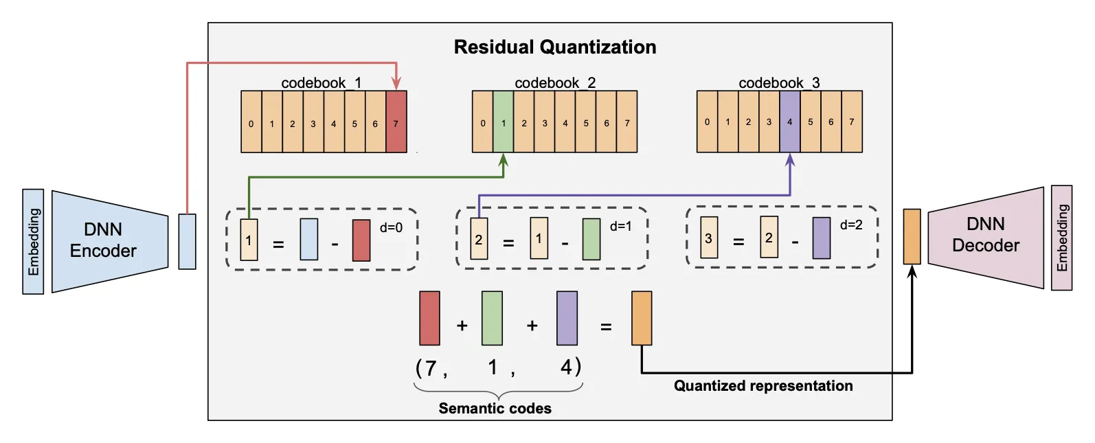
Semantic IDs (SIDs) are discrete codes that identify an element of the input space. Concretely, “codes” are indices along the codebook-size dimension of the codebook. Let $C$ be the codebook size (i.e., the number of vectors in the codebook), and $N$ be the SID’s latent dimension size; then each codebook is a $C \times N$ matrix over the real field. The vector-quantized variational autoencoder (VQ-VAE) maps a given element in the input space to a single code. The modern residual quantization variational autoencoder (RQ-VAE) uses a tuple of $D$ codes, stacking $D$ codebooks. It forms the SID tuple by taking an index from each layer. Quantization begins from the latent embedding itself, $\boldsymbol{r}_0 = \boldsymbol{z}$. Each codebook recursively quantizes the residual from the previous level, according to

$$k_d = \mathrm{quantizer}(\boldsymbol{r}_d), \quad \boldsymbol{r}_{d+1} = \boldsymbol{r}_d - \boldsymbol{e}^{(d)}_{k_d}, \qquad d = 0, \dots, D-1,$$

where $\boldsymbol{r}_d$ is the residual entering depth $d$, $k_d$ is the code selected from the $d$-th codebook, and $\boldsymbol{e}^{(d)}_{k_d}$ is the corresponding latent vector in that codebook. Concretely, the lookup is nearest-neighbor within the codebook:

$$k_d = \arg\min_{k \in \{0,\dots,C-1\}} \big\lVert \boldsymbol{r}_d - \boldsymbol{e}^{(d)}_{k} \big\rVert_2.$$

Stacking codebooks like this increases representational capacity exponentially, while memory footprint remains linear. SIDs can be either unique to a corpus element or non-unique by design. TIGER appends an additional unique identifier code to all SIDs that collide. PLUM argues that SID collision is a feature, not a bug. Latent code vectors group embeddings into clusters. Codebooks achieve peak uniformity in code utilization when the latent code vectors are the embeddings’ cluster centroids (GRID). SIDs are thought of as semantically coarse-to-fine with depth. The $d=0$ level is the most general, while later depths represent increasingly fine details.

2.3 Generative Recommendation

GR’s advantage is its superior capacity to capture inter-item semantics (GenRet). An item is the base unit of a GR dataset. For the Amazon Reviews 2023 Dataset, an item is a catalog product sold on the Amazon.com e-commerce platform. Sequences string together items in a semantically meaningful way. For Amazon Reviews, de-identified users’ purchase histories serve this purpose.

Autoregressive GR models learn the task via maximum likelihood estimation on the target recommendation: a held-out SID. They commonly use beam-search decoding to output the top-$k$ items to recommend. Decoding is simultaneously retrieval and reranking. Recall (or hit rate) and Normalized Discounted Cumulative Gain (NDCG) are the critical metrics under consideration on validation and test splits. Both the retrieval and ranking targets are a single item (the SID held out in the sequence). Recall then indicates the proportion of sequences for which the model correctly recovers the target in its top-$k$ lookup. NDCG accounts for the position of the retrieval target in the top-$k$, i.e., how well the model ranks.

3. Method

We adopt the embedding hit rate and Gini coefficient proxy metrics proposed by FORGE. The core track consists of: a Qwen 3.5 0.8B-parameter instruct-initialized VLM for embedding model experiments, and an RQ-VAE with codebook depth $3$, size $256$, and latent dimension $64$. We borrow these parameters from literature precedent on datasets of similar magnitude and complexity (namely, Amazon Reviews). To evaluate a given vocabulary’s efficacy, we train a T5 encoder-decoder transformer (GRID, TIGER) on the generative recommendation (GR) task in a configuration held constant across all upstream variations. Experiments run to convergence via early stopping on their proxy metric.

3.1 Dataset

OpsVerse is a set of executed work-order operations (ops) and a co-occurrence signal. The VLM used in experiments consumes executed ops as images and HTML text. The raw data undergoes several decluttering and normalization transformations.

Co-occurrence is a similarity signal. Intuitively, we think of collections as “baskets” (or sequences) of “items.” Two items co-occur (i.e., are similar) if they appear together in any basket. The basket-item graph is bipartite (one set of vertices for baskets, the other for items). An edge exists between vertices when a basket contains an item.

We materialize the co-occurrence signal in OpsVerse as follows. The unit items are executed ops. Two executed ops co-occur iff their parent template ops appear together in a template. A template op is represented implicitly by its op-content: a SHA-256 hash of the content that lets us trace an executed op back to its parent template op. Executed ops are then variations, or augmentations, of their template op.

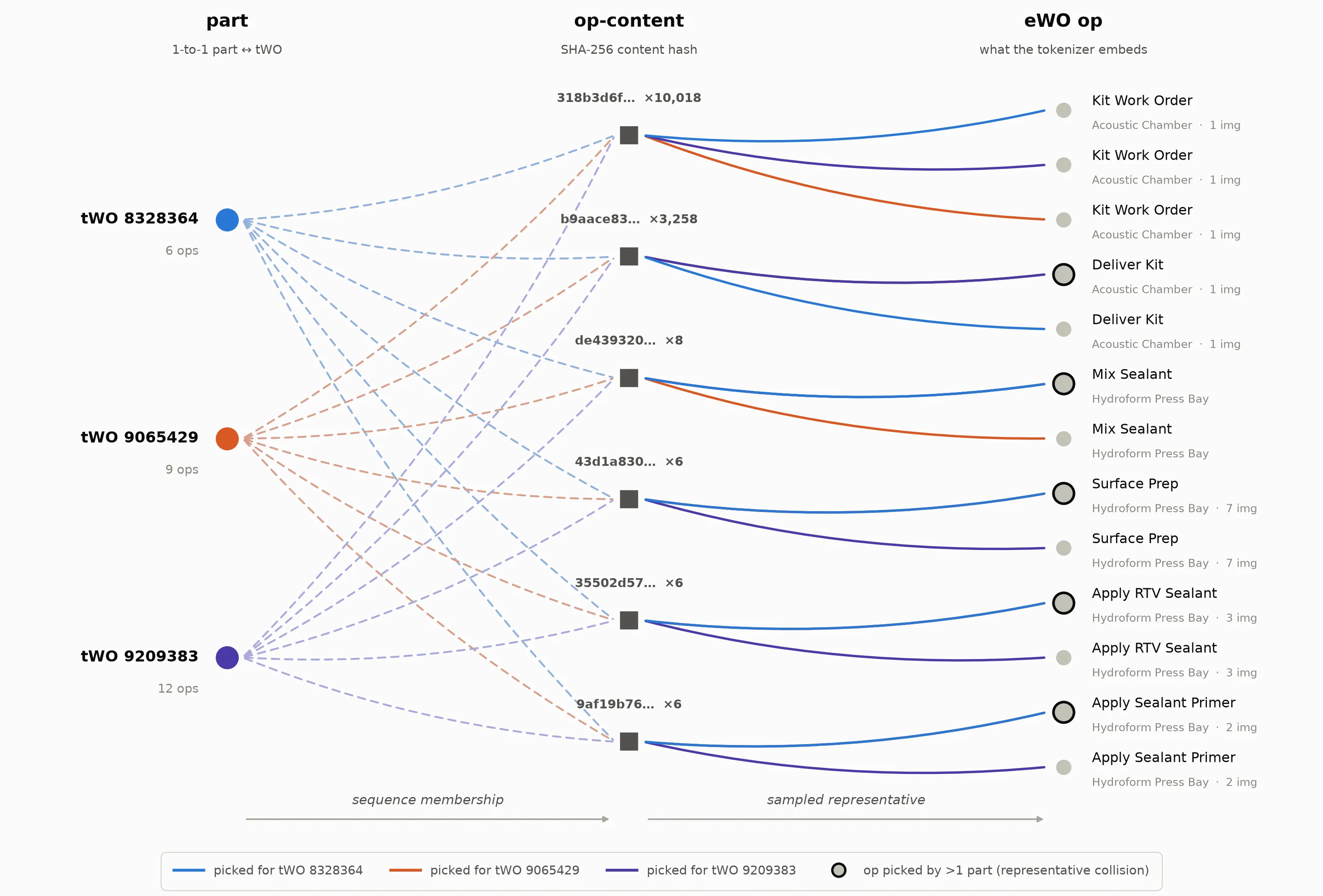
Template ops are uniquely distinguished by their op-content hashes. We use “op-content” interchangeably with “template op”. Op-contents are reused across templates, producing the bipartite structure we need to form the co-occurrence signal. A reduction is performed over the executed ops that map to the same op-content by sampling a different one for each occurrence of the op-content across part templates. The final result is one executed op per (part, op-content). The sampled executed op is the representative.

The final bipartite graph undergoes 5-core filtering. 5-core filtering iteratively drops operations until it reaches a steady state according to the rule: a (part, op-content) is kept iff the content appears in $\ge 5$ templates and all templates contain $\ge 5$ different op-contents. 5-core ensures all remaining sequences are length $\ge 5$ and all remaining items appear in $\ge 5$ other sequences.

Notice that if we model operation items as vertices and place edges between all executed ops iff they co-occur, we form the co-occurrence graph of the OpsVerse data. The graph naturally forms clusters of nodes around operations commonly seen together in work orders. A hub operation might be a menial task that’s required for the construction of many different parts. E.g., cleaning up after assembling a tube in the tube shop is common across many tube-assembly work orders. It may seem ill-conceived, given that this biases the signal toward over-representing hubs, but it is by design. Cleaning up after oneself is an expected behavior in many contexts and is therefore a reasonable recommendation. That said, co-occurrence’s only purpose is to finetune an embedding model to bolster downstream generative recommendation. It is not the foundation of the system’s recommendation ability.

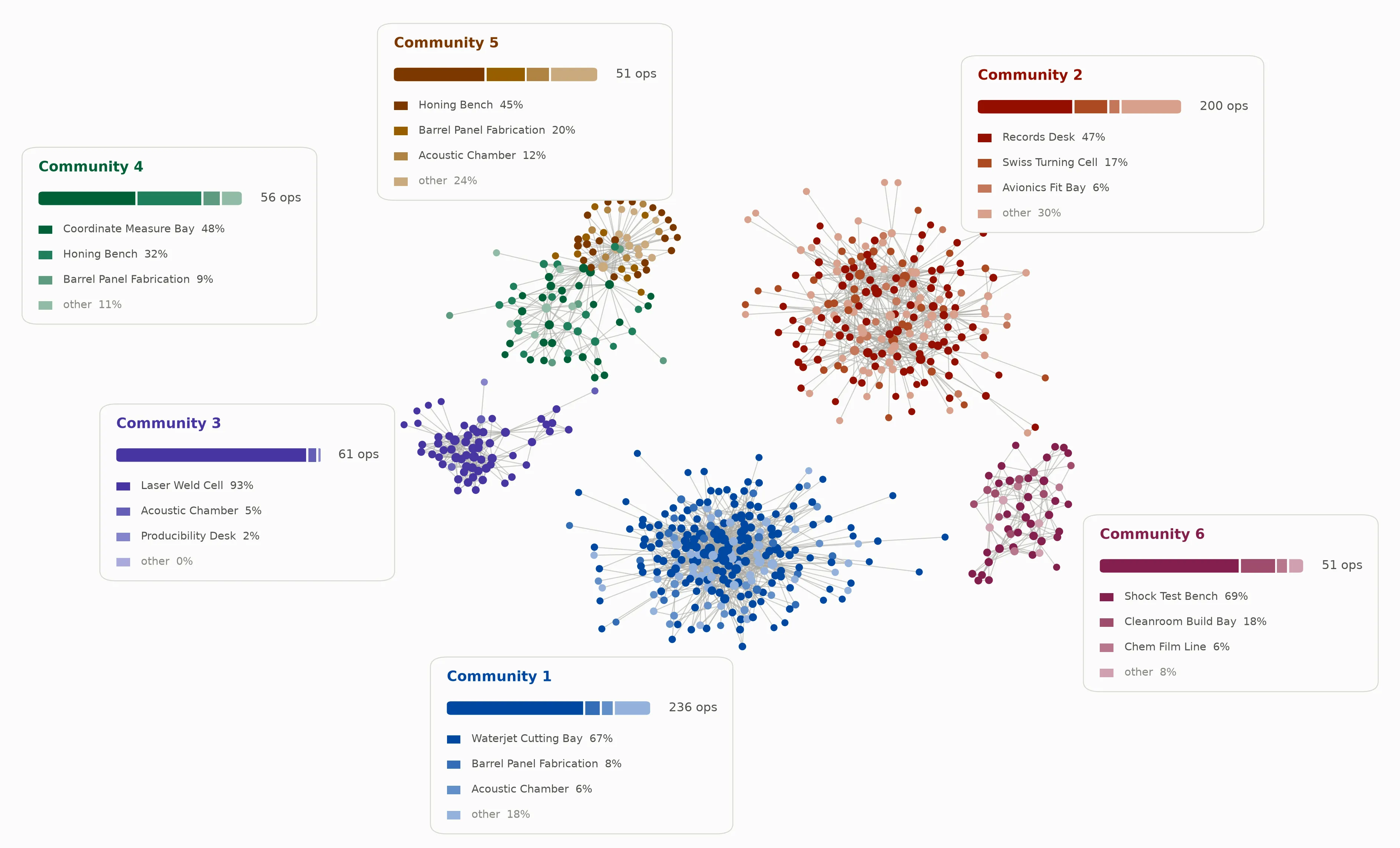
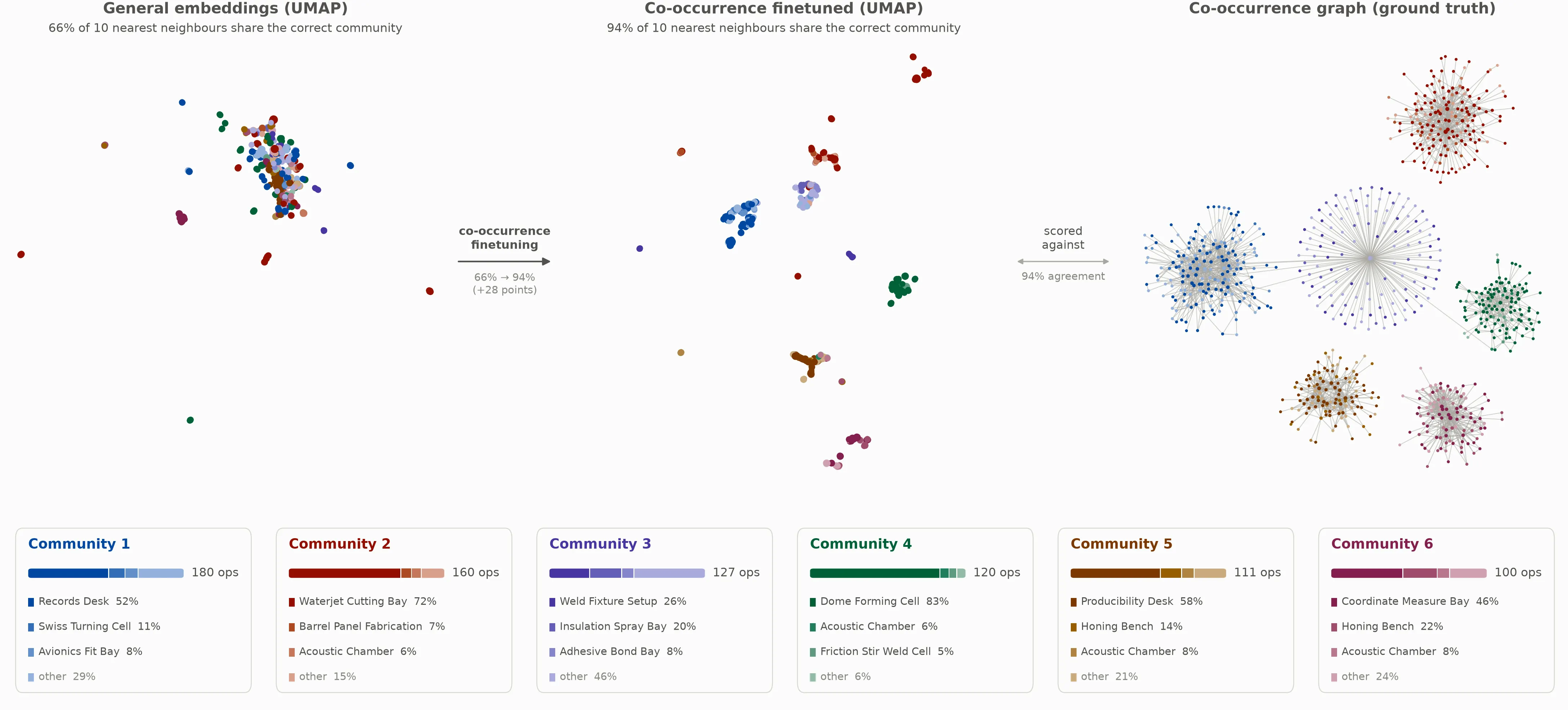
We find it helpful to attach a more intuitive taxonomy grouping to the OpsVerse co-occurrence graph. Our taxonomy of choice is the operation’s work center. There are over a hundred unique work centers. Some examples include Tube Shop, Metallic Post Processing, Inventory, and Composites.¹Work-center names here and in all figures are fictitious stand-ins that resemble real rocket work centers. Real names are withheld for confidentiality. We also introduce a labeling system called communities. Communities are formed by running infomap, a community-detection algorithm, on the co-occurrence graph. At a high level, the algorithm establishes community partitions by determining how to compress random-walk trajectories into minimal-length descriptions. Hence, encoding a step within a community is cheap, and encoding a transition between communities is expensive. A set of communities scores well when the walks tend to linger inside the partitions. These partitions are then densely-connected groups of operations. Figure 4 illustrates the top 6 largest communities, and the top 3 most prominent taxa by community. Note that lines between communities are drawn arbitrarily, and work-center taxonomies offer a human-friendly category to latch onto. Neither necessarily captures the graph’s structure. Nor do the two methods always align. Taxonomies and communities are qualitatively useful and are at least correlated with the desired semantic structure co-occurrence is intended to instill.

From the OpsVerse set, two kinds of splits are produced: item-wise and sequence-wise. A $0.10$ threshold on a uniform continuous hash $\in [0, 1]$ of an operation’s content determines whether the operation item belongs to the item-wise held-out validation split. A sequence-wise split is formed by masking the end elements of the input sequence. GR models consume the SID sequence, with the second-to-last element held out for the validation split and the last element for the test split. Table 1 summarizes the final dataset.

Table 1. OpsVerse dataset statistics. Sequences are part templates; interactions are (part, op-content) cells, each carrying one representative executed op. The item-wise held-out items are withheld from embedding-model and quantizer training.

Statistic	Value
Unique Items (executed ops)	101,860
Sequences (part templates)	24,121
Interactions	319,909
Interaction density	$1.30 \times 10^{-4}$
Op-contents (post-5-core)	7,435
Distinct work centers	113
Sequence length (mean / median / min / max)	13.26 / 12 / 5 / 80
Instruction text chars (mean / median)	1,810 / 1,297
Items with $\ge 1$ image	23.9%
Item-wise held-out items	10,186 (10.0%)
Distinct validation / test targets	10,417 / 9,129

3.2 Embeddings

We explore finetuning with a contrastive co-occurrence signal (FORGE, PLUM) on the OpsVerse items. The items consist of semantically related text and images. We explore the full Cartesian product of $\{\text{text + images},\text{text-only}\} \times \{\text{Full SFT}, \text{LoRA}\}$. Doing so implicitly navigates the finetuning’s capacity to alter the initialized model’s representation. Including images with text requires that the finetuning method can induce sufficient change in representation to model how image features relate to the co-occurrence signal. Full supervised finetuning presents the maximum capacity to alter embedding representation. LoRA presents decreased capacity proportional to rank. So theoretically, text + images is expected to require greater capacity than text-only, and full SFT provides greater capacity than LoRA.

Our approach to LoRA follows Thinking Machines’ LoRA Without Regret. We use adapters for all weight matrices. We measure OpsVerse’s information density (via their estimate of $\approx 1$ bit/token), then use the $2$-bits/param recommendation to select a rank $r$ of $16$ without sweeping. LoRA scaling factor $\alpha$ is rescaled by $\frac{1}{r}$ to be rank-independent. The remaining parameters are taken from HuggingFace’s peft library defaults, which Thinking Machines were unable to improve on.

Prior work showed that contrastive learning is most effective when provided with many negative examples (SimCLR, Wang & Isola 2020). For all embedding model experiments, we implement a global batch size of $2048$ using GradCache (VLM2Vec).

We finetune with the OpsVerse co-occurrence signal via gradient descent on NT-Xent. Embedding model experiments are evaluated on the embedding hit rate (FORGE) proxy metric as follows,

$$\text{EmbHitRate@}k = \frac{1}{\lvert \mathcal{Q} \rvert}\sum_{q \in \mathcal{Q}} \frac{\lvert \mathcal{R}_q \cap \text{top-}k(q) \rvert}{\lvert \mathcal{R}_q \rvert},$$

where $\mathcal{Q}$ is the set of embedding queries and $\mathcal{R}_q$ is the set of all co-occurrence neighbors for query $q$. Embedding hit rate measures the mean proportion of co-occurrence graph neighbors retrieved in an embedding’s $k$ nearest neighbors. It quantifies how well proximity in embedding space represents the co-occurrence graph and has been shown to correlate strongly with downstream GR performance (FORGE).

3.3 Quantization

When a source VLM embedding model completes finetuning, it performs an additional inference pass on the OpsVerse items. Those embeddings are stored and become raw data for the quantization stage.

Producing SIDs optimal for GR is challenging. Simplistic methods tend to suffer from codebook collapse, where embeddings quantize to one or few codes. Dead codes are then codes that are not utilized or are seldom utilized. Recommendation with a collapsed codebook is trivial, inflating apparent model performance. The optimal codebook has high utilization while capturing semantic signal relevant to the downstream GR task (FORGE).

All quantizer variants are subject to k-means clustering initialization and dead-code restarting. These techniques have shown consistent positive results (LMIndexer, GenRet, TIGER) and have little downside. K-means initialization involves initializing the quantizer’s codebook from a k-means fit of the training set. First, RQ-VAE’s FFN projects embeddings into the codebook dimension. For Qwen 3.5 0.8B, that means $1024 \rightarrow 64$. Then, we apply Lloyd’s algorithm with $256$ clusters, i.e., as many clusters as there are codebook vectors, then repeat on residuals for all $3$ codebooks. This variation is specifically rk-means (QARM). This gives the codebook a stable warm start, removing the need to initialize at random. For dead-code restarts, training maintains an exponential moving average (EMA) of the in-batch cluster size for each code (initialized to $1.0$ with a decay of $0.99$). In-batch cluster size is the count of embeddings that map to the code during quantization. Each code’s corresponding EMA buffer updates every training step. When its EMA falls below the threshold $10^{-4}$, we restart the code, sampling a random latent from the step’s batch to replace the dead code’s latent vector.

The remaining design heuristics we explore present non-linear interaction effects. We sweep the space,

$$\begin{aligned} &\{\text{EMA},\ \text{gradient}\} && \text{codebook update} \\ &\times\ \{\text{STE},\ \text{rotation trick}\} && \text{gradient propagation} \\ &\times\ \{\text{none},\ \text{standardization},\ \text{ZCA}\}. && \text{feature scaling} \end{aligned}$$

Gradient codebook updates are computed with respect to the reconstruction term, which measures how well the decoding FFN $g(\cdot)$ recovers the embedding $\boldsymbol{x}$ from the latent code $\hat{\boldsymbol{z}}$,

$$\hat{\boldsymbol{z}} = \sum^{D-1}_{d=0} \boldsymbol{e}^{(d)}_{k_d}, \qquad \mathcal{L}_{\text{recon}} = \big\lVert \boldsymbol{x} - g(\hat{\boldsymbol{z}})\big\rVert_2^2,$$

as well as a codebook loss term that pulls each level’s selected code toward the vector it approximates,

$$\mathcal{L}^{(d)}_{\text{codebook}} = \big\lVert \mathrm{sg}[\boldsymbol{r}_d] - \boldsymbol{e}^{(d)}_{k_d} \big\rVert_2^2,$$

where $\mathrm{sg}[\cdot]$ is the stop-gradient operator and $\boldsymbol{r}_d$ is the residual the level quantizes.

EMA codebook updating replaces the gradient step on $\mathcal{L}_{\text{codebook}}$ with an online Lloyd’s algorithm step. Let $\mathcal{B}^{(d)}_k$ be the set of level-$d$ residuals mapped to code $k$ within the batch. We track two EMAs per code: one of the assigned vector sum, the other the assignment count.

$$\boldsymbol{m}^{(d)}_{k} \leftarrow \gamma\, \boldsymbol{m}^{(d)}_{k} + (1-\gamma) \sum_{\boldsymbol{r} \in \mathcal{B}^{(d)}_{k}} \boldsymbol{r}, \qquad n^{(d)}_{k} \leftarrow \gamma\, n^{(d)}_{k} + (1-\gamma) \big|\mathcal{B}^{(d)}_{k}\big|,$$

and update the code to their ratio,

$$\boldsymbol{e}^{(d)}_k \leftarrow \frac{\boldsymbol{m}^{(d)}_k}{n^{(d)}_k},$$

where $\gamma$ is the decay rate. Code latent vectors track the running mean of the embeddings assigned to them. MTGRec reports that this method is more effective than gradient descent for codebook learning.

The RQ-VAE encoder latent $\rightarrow$ codebook latent lookup step is non-differentiable. As is typical, we implement straight-through gradient estimation (STE) via a clever tensor detachment, to circumvent the computation graph break:

# e: FFN encoder latent (requires grad). q: selected latent codebook vector.
q = e + (q - e).detach()

STE transplants the backward pass gradient across the codebook. STE is a design decision, an inductive bias. Higher-fidelity gradient estimation methods exist. However, as an estimator approaches differentiability, the system approaches an autoencoder. Autoencoders generalize poorly and tend to overfit (Rotation Trick). If we disregard the reconstruction loss, STE applies the same gradients to all encoder latents that map to a given code (the Voronoi cell). The rotation trick is an alternative approach to gradient estimation that lets gradients tune based on $\boldsymbol{e}$‘s location within the cell, increasing granularity. The rotation trick replaces the identity transform with a rotation-and-rescale one, carrying $\boldsymbol{e}$ onto $\boldsymbol{q}$,

$$\boldsymbol{q} \leftarrow \mathrm{sg}\!\left[\frac{\lVert \boldsymbol{q} \rVert}{\lVert \boldsymbol{e} \rVert} \boldsymbol{R}\right] \boldsymbol{e}, \qquad \frac{\partial \mathcal{L}}{\partial \boldsymbol{x}} = \frac{\partial \mathcal{L}}{\partial \boldsymbol{q}} \frac{\lVert \boldsymbol{q} \rVert}{\lVert \boldsymbol{e} \rVert}\boldsymbol{R} \frac{\partial \boldsymbol{e}}{\partial \boldsymbol{x}},$$

where $\boldsymbol{R}$ is computed via Householder matrix reflections.

Feature scaling data preprocessing is used throughout machine learning to remove first- and second-order structure from a distribution. We consider three settings on the quantizer’s input. Let $\boldsymbol{\mu}$ and $\boldsymbol{\Sigma}$ be the mean and covariance of the projected embeddings, estimated over the training set. With “none” whitening, the raw projected embedding is quantized directly. Standardization centers and rescales each dimension independently,

$$\tilde{\boldsymbol{z}} = \mathrm{diag}(\boldsymbol{\Sigma})^{-1/2} (\boldsymbol{z} - \boldsymbol{\mu}).$$

Zero-phase component analysis (ZCA) whitening instead applies the full transform

$$\tilde{\boldsymbol{z}} = \boldsymbol{A}^{-1/2} (\boldsymbol{z} - \boldsymbol{\mu}), \qquad \boldsymbol{A}^{-1/2} = \boldsymbol{U} \boldsymbol{\Lambda}^{-1/2} \boldsymbol{U}^{\top},$$

for $\boldsymbol{U}$ orthonormal, $\boldsymbol{\Lambda}$ diagonal from the eigendecomposition. ZCA is similar to PCA in that they both decorrelate and enforce unit variance. But ZCA appends the inverse rotation to $\boldsymbol{U}^\top$, which can be shown to minimize L2 w.r.t. the pre-transformed data ($\lVert (\boldsymbol{z} - \boldsymbol{\mu}) - \tilde{\boldsymbol{z}} \rVert_2$). MTGRec reports that representation whitening improves SID quality.

We navigate the quantization design space via a screen with a proxy metric, then promote the top 3 configurations to full GR evaluation. The Gini coefficient is our proxy metric. Let $a^{(d)}_{i}$ be the usage count for SID $i$ in $\mathcal{S}^{(d)}=\{s_1, \dots, s_{N_d}\}$, ordered ascending by usage count for the level-$d$ codebook, then

$$A(i) = \sum^i_{j=1}a^{(d)}_j, \qquad \text{Gini}_d=\frac{2}{N_d}\sum_{i=1}^{N_d} \left(\frac{i}{N_d}-\frac{A(i)}{A(N_d)}\right).$$

The Gini coefficient is based on the Lorenz curve and indicates code-usage fairness. For the screen sweep, we compare the worst $\text{Gini}_d$ (i.e., its upper bound) over codebooks:

$$\text{Gini} = \max_d \text{Gini}_d.$$

3.4 Generative Recommendation

To fairly evaluate OpsVerse embeddings and their learned quantizations, we follow TIGER and GRID’s precedent with minor deviations. The GR model is a T5 encoder-decoder transformer. We decode via unconstrained beam search. As a result, the autoregressive model may produce discrete code tuples with no corresponding item. A hit is a verbatim match to the ground-truth code tuple. This approach minimizes metric bias. For example, constraining beam search to existing SIDs would artificially inflate recall and reward low codebook utilization. Decoding is restricted to 3 steps (no EOS token), and the input sequence has separator tokens inserted between codes. We deviate from TIGER by not appending a unique integer to codes to avoid collisions. Instead, we adopt PLUM’s philosophy that collisions are a feature in recommendation. Accepting collisions simplifies and further debiases the model. It places the burden of semantic representation on SIDs, preventing the T5 from having to model both inter-item relations and SID-item ownership. We report the Recall@$\{5, 10\}$ and NDCG@$\{5, 10\}$ of the final top-3 GR models produced from the SID configurations that pass the screen.

4. Experiments

4.1 Embeddings

Embedding model experiments begin with a factorial sweep of text + image versus text-only OpsVerse items, together with full supervised finetuning versus LoRA. For text-only, images are stripped in-place. Their surrounding text remains. The motivating hypothesis for excluding images is that the surrounding text describes them. The images might be redundant with respect to the information they offer to co-occurrence signal modeling. Excluding images reduces the memory footprint and removes their quadratic contribution to sequence length.

Interestingly, Table 2 shows that all embedding model variants plateau around the same embedding hit rate performance. LoRA sees a slight boost. Meanwhile, including images is mixed. But realistically, all configurations are within noise of each other. This behavior is an unintuitive result. It suggests that an EmbHitRate@$100$ of $\approx 0.5$ is the maximum achievable on the OpsVerse dataset as it is presently curated. Importantly, the metric is not saturated: the random-retrieval floor is $\approx 0.0244$, and the validation-split ceiling is $\approx 0.9998$,²The floor assumes random retrieval: let $n=4096$ be the subsampled validation split size, $\mathcal{A}$ be its anchors, $T_a$ be the $k=100$ retrieved randomly for $a$, $\mathcal{R}_a$ the co-occurrence neighbors for $a$, then$$\begin{aligned} &\mathbb{E}_{T_a} \mathbb{E}_{a \in \mathcal{A}}\left[ \frac{\lvert \mathcal{R}_a \cap T_a \rvert}{\lvert \mathcal{R}_a \rvert} \right]\\[0.5em] &\quad= \frac{1}{\lvert \mathcal{A} \rvert} \sum_{a \in \mathcal{A}} \frac{\mathbb{E}_{T_a}\lvert \mathcal{R}_a \cap T_a \rvert}{\lvert \mathcal{R}_a \rvert}\\[0.5em] &\quad= \frac{1}{\lvert \mathcal{A} \rvert} \sum_{a \in \mathcal{A}} \frac{1}{\lvert \mathcal{R}_a \rvert} \frac{k \lvert \mathcal{R}_a \rvert}{n-1}\\[0.5em] &\quad= \frac{k}{n - 1}. \end{aligned}$$The ceiling assumes perfect retrieval, where every anchor’s co-occurrence neighbors are ranked ahead of all non-neighbors, computed:$$\mathbb{E}_{a \in \mathcal{A}} \left[ \min \left(1.0, \frac{k}{\lvert \mathcal{R}_a \rvert} \right) \right].$$$\min(\cdot,\cdot)$ handles the case where $\lvert \mathcal{R}_a \rvert \le k$ so hit rate $=1.0$ and where $\lvert \mathcal{R}_a \rvert > k$ so hit rate $= k / \lvert \mathcal{R}_a \rvert$. so the plateau sits at roughly half the attainable range. Surpassing it requires further investigation into its source.

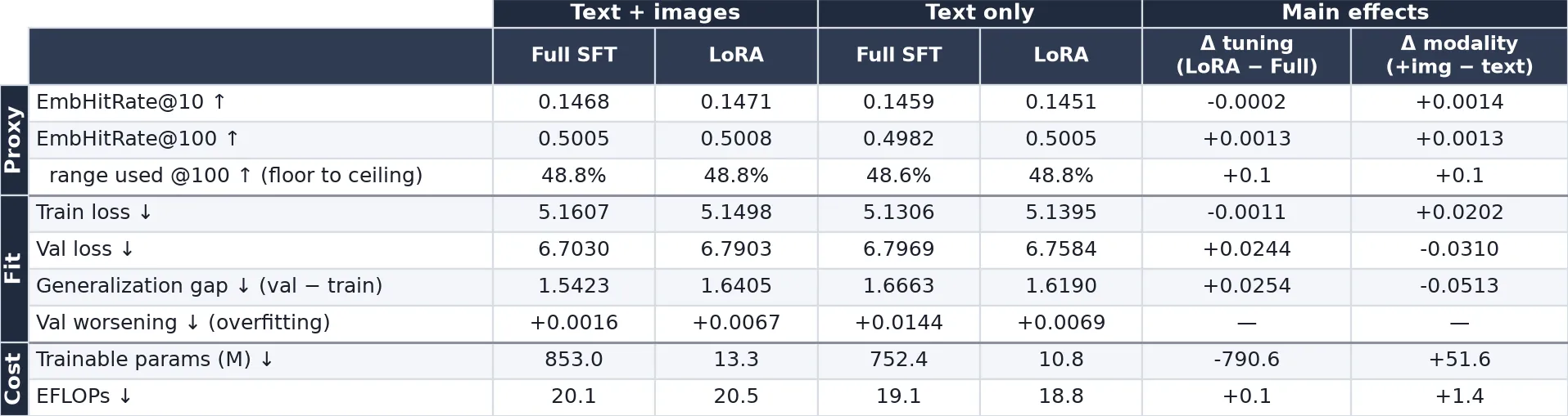
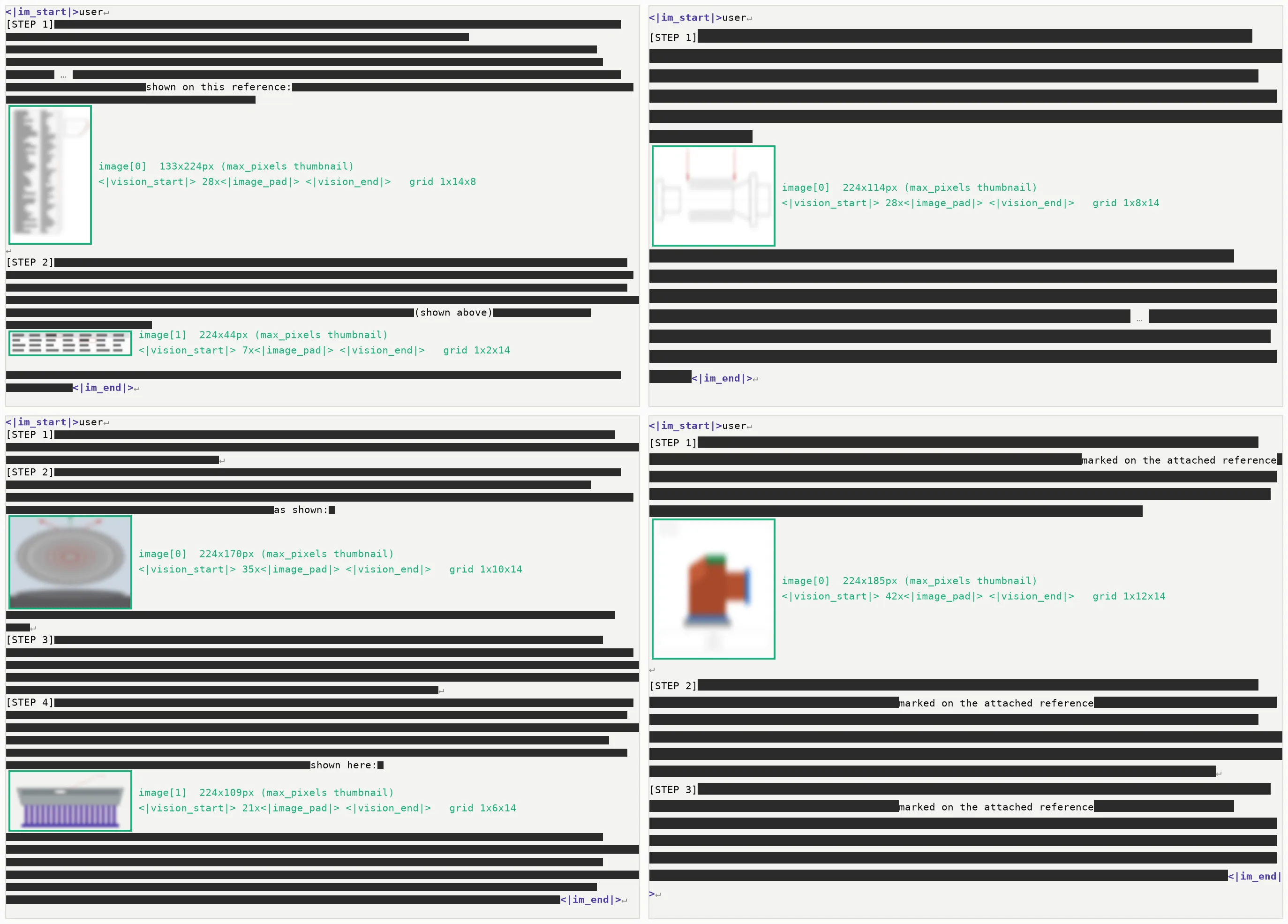
That said, we choose to adopt both LoRA finetuning and text + image modalities moving forward. As shown in Table 2, LoRA has hundreds of millions fewer trainable parameters, freeing VRAM for a larger chunk size and reducing training time. For images, we provide a qualitative argument. Looking closely at the item examples in Figure 2, we see language to the effect of “as shown below.” The OpsVerse operations are engineering documents with diagrams that tend to contain information exclusive to them. The images are therefore not overtly redundant. Context is incomplete without them. In addition, only $23.9\%$ of items contain images, and the images are constrained to $224 \times 224$ (a potential culprit for the lack of performance gain from including them). So the prospective memory reduction is marginal. We concede the +1.4 exaFLOPs and +51.6M trainable parameter increases (excluding images means no vision tower).

Although not included in the table, we observe the same plateau after scaling up with a general-purpose, embedding-initialized Qwen 3 VL. Despite the mysterious performance plateau, co-occurrence finetuning significantly increases agreement between the embedding space and the co-occurrence graph. Figure 5 presents a UMAP before-and-after of a general-purpose embedding initialization with text + image LoRA finetuning. Starting from $66\%$ agreement (undoubtedly from clumping all items together), co-occurrence finetuning increases graph agreement to $94\%$. Side-by-side comparison with the co-occurrence graph illustrates the improvement.

4.2 Quantization

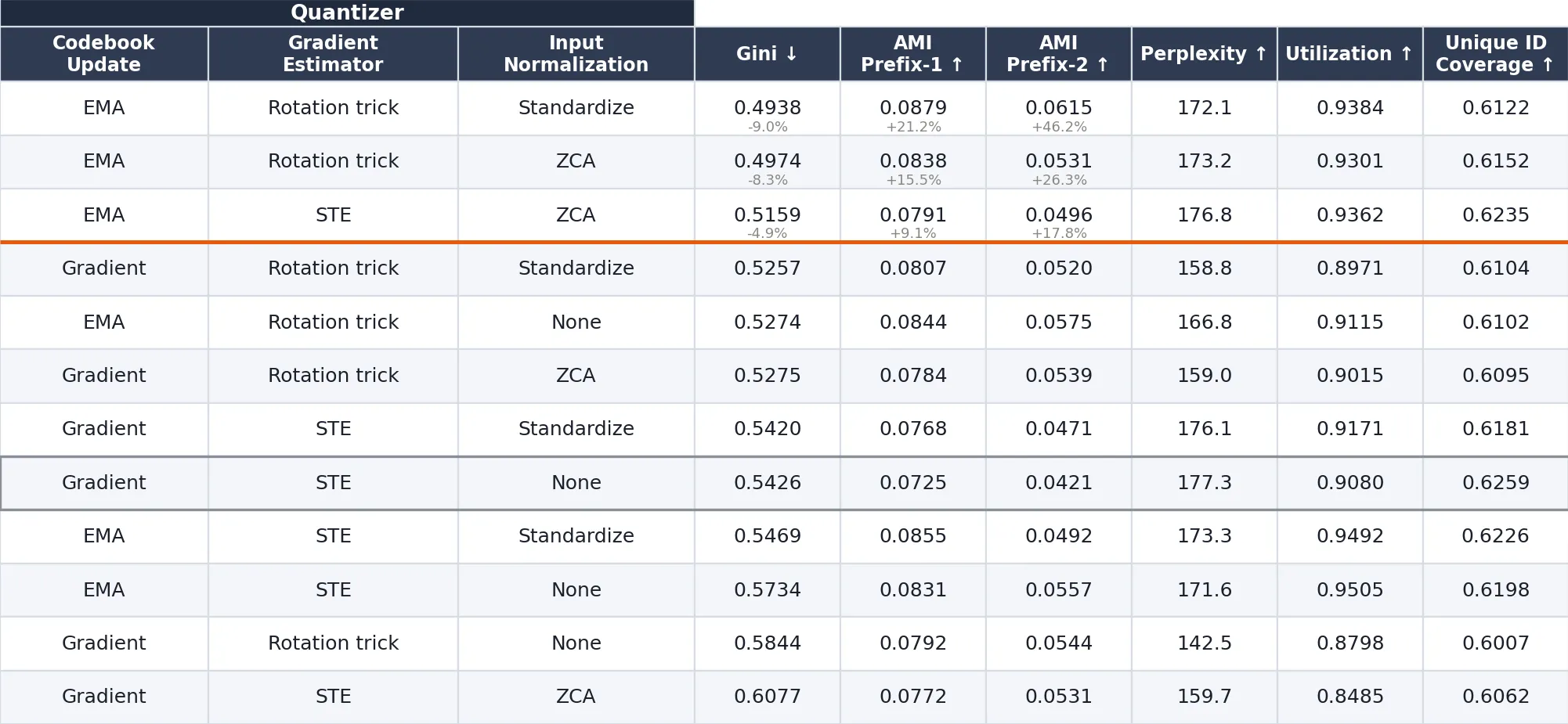
The goal of quantization is to produce a meaningful semantic vocabulary for the downstream recommender. But full GR training is expensive, so we perform the full 12-configuration sweep as a proxy metric screen. RQ-VAE learns multi-codebook SIDs. Therefore, every codebook has its own Gini coefficient. We monitor and report the upper bound of the Gini coefficient across codebooks. Table 3 shows the results of the quantizer configuration sweep. The top 3 configurations are promoted for full GR evaluation.

Table 3 also includes additional codebook metrics. Perplexity, utilization, and unique ID coverage are all indicators of codebook health. They exist to signal codebook collapse. All 12 configurations hold steady across them. Adjusted mutual information (AMI), a clustering-agreement score, measures how well the learned codes represent the taxonomy groupings at a given prefix length. AMI prefix-1 and prefix-2 indicate that the top-Gini SIDs successfully model coarse-to-fine semantic structure. They show improvement over the baseline by as much as $21.2\%$ and $46.2\%$, respectively.

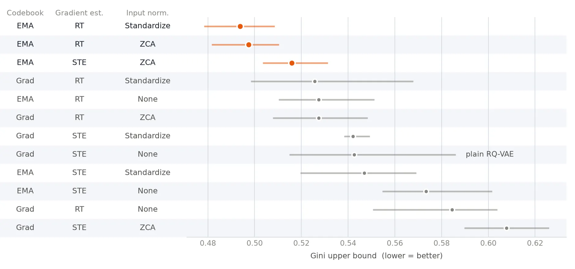
Furthermore, Figure 6 is a whisker plot of the same 12 configurations, ordered by Gini (upper bound). It highlights the necessity of a systematic sweep of codebook configurations. Had we pursued a greedy incremental approach, we might have excluded certain techniques for underperforming the baseline. For instance, if we took the baseline plain RQ-VAE and only switched STE for the rotation trick (the second-to-worst configuration), we may have dismissed the rotation trick altogether.

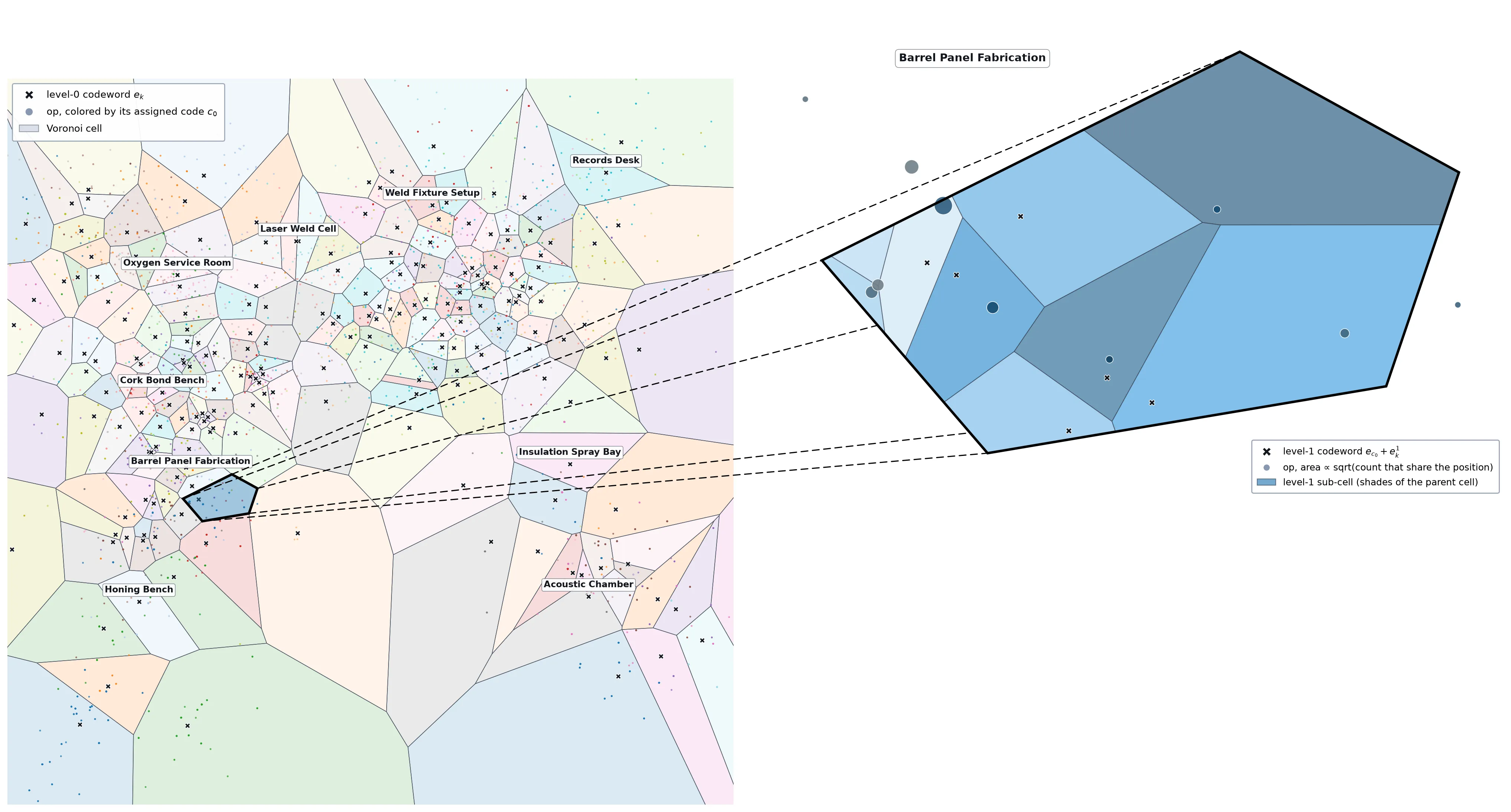
The Voronoi diagram in Figure 7 visualizes the level-0 learned codebook. It renders certain taxonomies more densely concentrated than others. Items in these regions appear to require higher granularity to differentiate those that co-occur. Perhaps operations from them have very similar co-occurrence behavior but differ significantly in content. That said, this analysis is largely tongue-in-cheek due to the projection limitations (mentioned in Figure 7’s caption) and the general abstractness of learned semantic embeddings.

4.3 Generative Recommendation

Table 4 shows the results of the top-3 quantizer configurations promoted to full GR model training and evaluation. ZCA whitening came out slightly ahead of regular standardization when supported by EMA codebook updates and rotation-trick gradient propagation. But the improvement is within noise. That said, choosing rotation-trick estimation over STE with EMA codebook updates and ZCA whitening does yield a meaningful improvement. Downstream recommendation performance may be robust to feature cross-correlation (ZCA decorrelates, standardization does not) under EMA updates, which is somewhat intuitive, but substantiating this claim would require further investigation.

Note that each promoted quantizer outperforms its popularity floor at $k=5$ but not $k=10$. The popularity floor is the baseline recall of always predicting the $k$ most frequent SID tuples from usage counts alone. It uses no generative model. Usage counts are codebook-dependent, and so they differ by quantizer. All three configurations beat the floor in the first $5$ beams, with (EMA, rotation-trick, ZCA) producing the largest relative improvement of $\approx 13\%$. But, at $k=10$ the advantage disappears, and even (EMA, rotation-trick, ZCA) essentially ties the floor ($-0.6\%$). Beams $6$–$10$ as marginal candidates only add $0.0501$ recall, while the popularity floor adds $0.0714$ ($\approx 43\%$ more). Beam search is known to produce low-diversity candidates that share prefixes (Diverse Beam Search). So later beams that share a length-$2$ prefix with earlier ones, yet carry an incorrect final code, earn nothing under verbatim matching. Candidates may correspond to no real item, or may be near duplicates of higher beams. On the other hand, the floor’s predictions are always valid, distinct, and high-frequency. That said, low diversity will still prove practically useful thanks to the SID’s coarse-to-fine prefix co-occurrence behavior. Constraining the beam search to retrieve SIDs corresponding to existing items also has practical upside but would bias evaluation (as explained in §3.4). Overall, the model’s inability to clear the floor at $k=10$ leaves room for improvement on the GR stage.

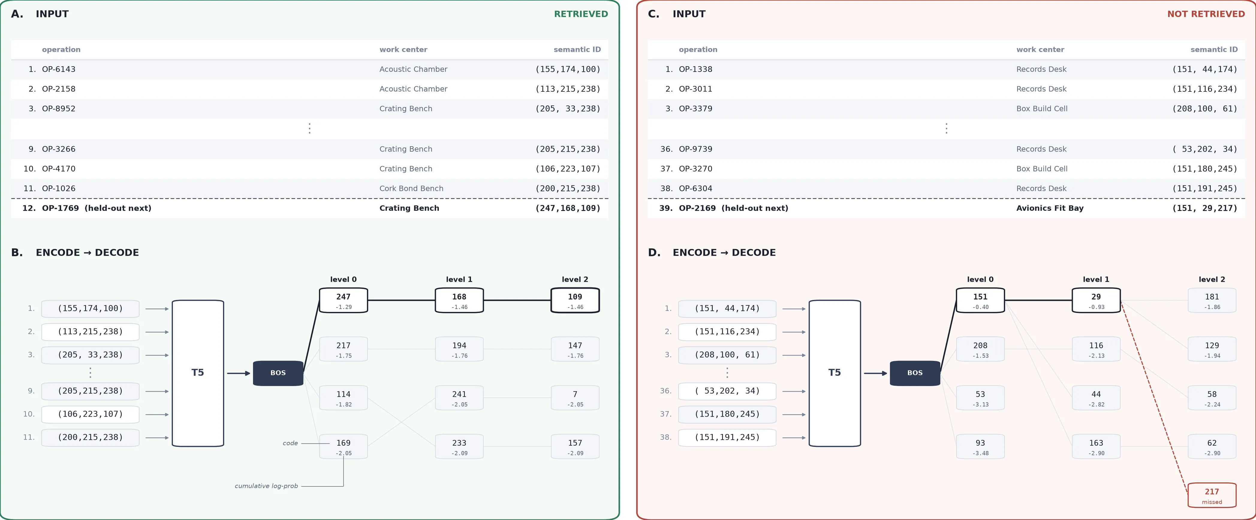
Figure 8 illustrates two real OpsVerse model inference examples: one in which the model successfully decodes the held-out operation, and another in which it misses the last target code. They are hand-picked, so of course, they are not indicative of model performance. Still, they summarize the study’s final artifact: a system that represents operations with semantic IDs and can recommend operations to add to work orders during their creation.

5. Conclusion

Traditional intuition assumes GR pipeline design changes produce predictable, stage-by-stage improvements. Our sweeps demonstrate this is not true in general. Work-order embeddings plateaued on the embedding hit rate proxy for GR performance independent of the included modalities and representation-altering capacity. The quantizer axis proved non-monotonic: the rotation trick underperforms the baseline in isolation but wins overall when combined with EMA updates and ZCA whitening. The Gini proxy screen’s ordering largely survived full GR evaluation, with one within-noise transposition.

More work is needed on OpsVerse GR. We need to investigate and address the source of the embedding model’s proxy metric performance plateau. We suspect it is a data limitation, so we should conduct data-related ablations. Perhaps we could lean into the idea that an executed op is an augmentation of its template op, and sample new executed ops for a given op-content at each epoch of the training split. There’s room to conduct quantizer Gini screening at a larger scale. It would also be worth promoting low-performing Gini screen configurations to full GR evaluation to confirm the proxy metric’s efficacy in global ranking. Cold-start performance could be more rigorously evaluated on OpsVerse under the embedding model finetuning regimes. We suspect that full SFT on the co-occurrence signal may partially degrade useful VLM priors that cold-start benefits from more than LoRA, because full SFT has greater capacity to alter the model’s latent representation. Lastly, the GR model itself could be relieved of its SID-evaluation role, perhaps by scaling and experimenting with other techniques to improve later-beam quality.

Overall, the study explores modern SID GR techniques on the OpsVerse GR dataset. SIDs bridge complex multimodal engineering documents, items with no native token representation, into unimodal, token-based generative modeling more broadly.

References

[1] Amazon Reviews 2023. Hou, Y. et al. “Bridging Language and Items for Retrieval and Recommendation.” ACL, 2026.

[2] Diverse Beam Search. Vijayakumar, A. K. et al. “Diverse Beam Search: Decoding Diverse Solutions from Neural Sequence Models.” AAAI, 2018.

[3] FORGE. Fu, K. et al. “FORGE: Forming Semantic Identifiers for Generative Retrieval in Industrial Datasets.” arXiv preprint arXiv:2509.20904, 2025.

[4] GenRet. Sun, W. et al. “Learning to Tokenize for Generative Retrieval.” NeurIPS, 2023.

[5] GRID. Ju, C. M. et al. “Generative Recommendation with Semantic IDs: A Practitioner’s Handbook.” CIKM, 2025.

[6] infomap. Rosvall, M. & Bergstrom, C. T. “Maps of Random Walks on Complex Networks Reveal Community Structure.” PNAS, 2008.

[7] LMIndexer. Jin, B. et al. “Language Models As Semantic Indexers.” ICML, 2024.

[8] LoRA Without Regret. Schulman, J. & Thinking Machines Lab. “LoRA Without Regret.” Thinking Machines Lab: Connectionism, 2025.

[9] MTGRec. Zheng, B. et al. “Pre-training Generative Recommender with Multi-Identifier Item Tokenization.” arXiv preprint arXiv:2504.04400, 2025.

[10] peft. Mangrulkar, S. et al. “PEFT: State-of-the-art Parameter-Efficient Fine-Tuning Methods.” GitHub repository, 2022.

[11] PLUM. He, R. et al. “PLUM: Adapting Pre-trained Language Models for Industrial-scale Generative Recommendations.” WWW, 2026.

[12] QARM. Luo, X. et al. “QARM: Quantitative Alignment Multi-Modal Recommendation at Kuaishou.” CIKM, 2025.

[13] Qwen 3.5. Qwen Team, Alibaba. “Qwen3.5-0.8B.” Hugging Face model card, 2026.

[14] Qwen 3 VL. Qwen Team, Alibaba. “Qwen3-VL-Embedding-2B.” Hugging Face model card, 2026.

[15] Rotation Trick. Fifty, C. et al. “Restructuring Vector Quantization with the Rotation Trick.” ICLR, 2025.

[16] RQ-VAE. Lee, D. et al. “Autoregressive Image Generation using Residual Quantization.” CVPR, 2022.

[17] SimCIT. Zhai, P. et al. “A Simple Contrastive Framework of Item Tokenization for Generative Recommendation.” arXiv preprint arXiv:2506.16683, 2025.

[18] SimCLR. Chen, T. et al. “A Simple Framework for Contrastive Learning of Visual Representations.” ICML, 2020.

[19] Straight-through estimation. Bengio, Y., Léonard, N. & Courville, A. “Estimating or Propagating Gradients Through Stochastic Neurons for Conditional Computation.” arXiv preprint arXiv:1308.3432, 2013.

[20] TIGER. Rajput, S. et al. “Recommender Systems with Generative Retrieval.” NeurIPS, 2023.

[21] VLM2Vec (MMEB). Jiang, Z. et al. “VLM2Vec: Training Vision-Language Models for Massive Multimodal Embedding Tasks.” ICLR, 2025.

[22] VQ-VAE. van den Oord, A., Vinyals, O. & Kavukcuoglu, K. “Neural Discrete Representation Learning.” NeurIPS, 2017.

[23] Wang & Isola 2020. Wang, T. & Isola, P. “Understanding Contrastive Representation Learning through Alignment and Uniformity on the Hypersphere.” ICML, 2020.

Citation

@article{ohanlon2026sids,
  author = {O'Hanlon, Charles},
  title  = {Work Order SIDs for Generative Recommendation},
  year   = {2026},
  month  = {aug},
  note   = {Blog post},
  url    = {https://charlescohanlon.com/blog/work-order-sids-for-generative-recommendation}
}

Footnotes

1. Work-center names here and in all figures are fictitious stand-ins that resemble real rocket work centers. Real names are withheld for confidentiality. ↩︎

2. The floor assumes random retrieval: let $n=4096$ be the subsampled validation split size, $\mathcal{A}$ be its anchors, $T_a$ be the $k=100$ retrieved randomly for $a$, $\mathcal{R}_a$ the co-occurrence neighbors for $a$, then

   $$\begin{aligned} &\mathbb{E}_{T_a} \mathbb{E}_{a \in \mathcal{A}}\left[ \frac{\lvert \mathcal{R}_a \cap T_a \rvert}{\lvert \mathcal{R}_a \rvert} \right]\\[0.5em] &\quad= \frac{1}{\lvert \mathcal{A} \rvert} \sum_{a \in \mathcal{A}} \frac{\mathbb{E}_{T_a}\lvert \mathcal{R}_a \cap T_a \rvert}{\lvert \mathcal{R}_a \rvert}\\[0.5em] &\quad= \frac{1}{\lvert \mathcal{A} \rvert} \sum_{a \in \mathcal{A}} \frac{1}{\lvert \mathcal{R}_a \rvert} \frac{k \lvert \mathcal{R}_a \rvert}{n-1}\\[0.5em] &\quad= \frac{k}{n - 1}. \end{aligned}$$

   The ceiling assumes perfect retrieval, where every anchor’s co-occurrence neighbors are ranked ahead of all non-neighbors, computed:

   $$\mathbb{E}_{a \in \mathcal{A}} \left[ \min \left(1.0, \frac{k}{\lvert \mathcal{R}_a \rvert} \right) \right].$$

   $\min(\cdot,\cdot)$ handles the case where $\lvert \mathcal{R}_a \rvert \le k$ so hit rate $=1.0$ and where $\lvert \mathcal{R}_a \rvert > k$ so hit rate $= k / \lvert \mathcal{R}_a \rvert$. ↩︎